Beyond probability – part-3

Answer to the question in part-2.

In theory, the method appears to stretch an extremely short event into a much longer observable time interval, allowing us to visualize events that occur far faster than ordinary human perception. However, there is a major practical limitation. To stretch a 1 microsecond event into 10 seconds, light itself must travel for about 10 light-seconds before returning. If the setup uses a round-trip path, that becomes approximately 20 light-seconds of total light travel distance.

Since light travels about 300,000 km per second, a 20-light-second path corresponds to roughly 6 million kilometers of optical path length. This is an enormous distance—far beyond the size of any laboratory. In fact, it is much greater than the average “Earth–Moon distance of about 384,000 km“. Because of this requirement, the idea is extremely difficult to implement as a practical measurement device, even though it remains an interesting thought experiment for understanding how time and observation can be transformed through the finite speed of light.

Thus, the concept is valuable for illustrating principles of observation and time scaling, but its physical implementation would require distances so large that it becomes impractical with present-day laboratory technology.

Now, starting part-3..

1] About a hidden variable not in the matchsticks

Imagine a person who has lived inside a completely sealed room since birth. Inside this room, there are scientific instruments, microscopes, lenses, and experimental setups. Over time, the person becomes skilled in using these tools and develops a strong scientific mindset. However, there is one absolute limitation: they have never seen the outside world. There is no knowledge of sunlight, no concept of day and night, and no awareness that anything exists beyond the room.

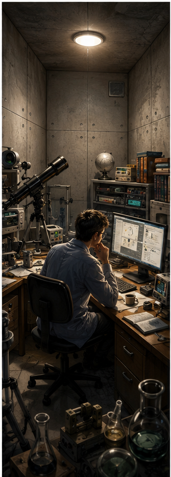
Within this confined environment, the person designs an experiment. A matchstick is placed at the focus of a lens, and the setup is taken outside briefly and then returned inside. This experiment is repeated every three hours, continuously, both during what would be day and night. From the experimenter’s perspective, each trial appears identical, because there is no awareness of external time or environmental variation.

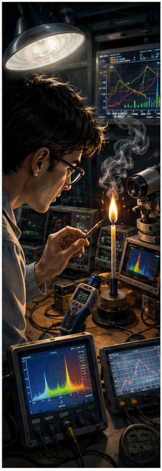
However, the outcome is not identical. In some cases, the matchstick burns, and in most cases, it does not. After a large number of repeated trials, the person begins to observe a pattern. Statistically, the matchstick burns approximately 10% of the time. Based on this data, a probability graph is constructed, and the system is described as having a 10% chance of success.

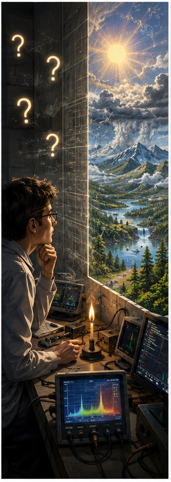
The person carefully examines every possible internal factor. The matchstick is inspected, the lens is analyzed, and the entire apparatus is checked for defects or inconsistencies. Despite this detailed investigation, no internal explanation is found. Everything inside the system appears consistent and identical across trials. As a result, the conclusion is drawn that there is no hidden variable within the system itself, and the observed behavior must be fundamentally probabilistic.

Even after accepting this result, a deep confusion remains. Why does the system produce only 10% successful outcomes? Why is it not consistently burning or consistently failing? From within the sealed framework of knowledge, the behavior appears random and irreducible. The probability becomes an accepted property of the system, rather than something to be explained.

Eventually, the person is taken outside the sealed environment. For the first time, they experience sunlight, observe day and night, and understand that external conditions change over time. After this exposure, a crucial realization emerges. The burning of the matchstick was not determined by any internal property of the matchstick or the lens, but by an external condition that was completely outside their previous field of knowledge.

The so-called randomness was not fundamental randomness. It was structured behavior governed by an external variable that was invisible within the original system. The “hidden variable” was not inside the experimental setup, but outside the boundary of what could be observed or even conceptualized.

This leads to a deeper insight. What is often called a hidden variable may not always be hidden within the object or system being studied. It may exist outside the accessible framework of observation itself. With limited instruments, limited senses, and limited theoretical models, such external causes may remain completely undetectable, even if they fully determine the outcome.

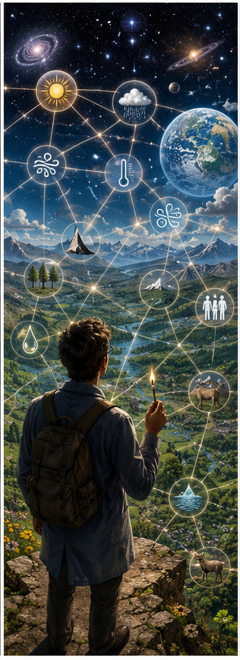
In extreme interpretations, it is even possible that some variables lie in domains of reality that are currently inaccessible, or not yet understood within our scientific framework. In such cases, the limitation is not in the phenomenon itself, but in the boundary of observation.

This creates a final reflection. When we search for hidden variables, we often assume they must be found within the system we are studying. But it is possible that the system is only a small part of a larger structure, and the true determining factors exist outside it. In that case, the search for hidden variables becomes constrained not by the absence of such variables, but by the limits of what we are able to perceive and define.

2] Understanding the probability wave

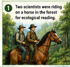
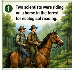
Two scientists entered the forest on horseback as part of an ecological reading and observation study.

While moving through the terrain, a sudden and powerful lion’s roar echoed across the forest. The sound triggered immediate panic in the environment.

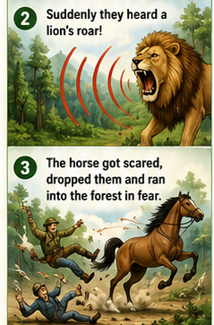
The horse they were riding became frightened and, in a sudden violent reaction, threw both scientists off its back. The horse then ran deep into the forest at very high speed driven purely by fear, without stopping, without hesitation, and without any return path.

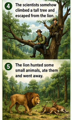
The scientists narrowly survived the chaos by climbing a tall tree nearby. From this elevated position, they observed the disturbance spreading through the forest while remaining safe from the lion. The lion briefly hunted smaller animals, fed, and then left the area, restoring silence once again.

After the forest stabilized, the scientists came down and began analyzing what had just happened. Their goal was no longer direct tracking, but reconstruction of motion from incomplete information. They built a probability model for the horse’s location inside the forest. Because the horse was moving under fear-driven conditions, its motion was assumed to be fast, directional, and non-returning. They estimated that the probability of finding the horse within a very small radius—such as within 5 km—was almost zero, because under panic it would not stop or reverse.

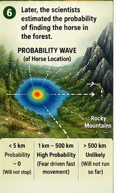
Instead, the probability spread across larger distances in structured pathways, with higher likelihood toward the rocky mountain region on the right side of the forest, where escape routes naturally converge. In this way, the horse was no longer a single traceable object in their view, but a time-dependent probability wave shaped by terrain, motion, and incomplete observation.

To resolve the uncertainty, a helicopter search was deployed by the forest department.

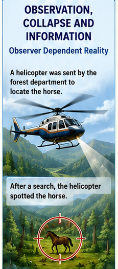
From above, the helicopter scanned large regions of the forest rapidly and eventually visually spotted the horse. At that moment, for the helicopter pilot, the entire probability distribution collapsed instantly into a single confirmed reality—the horse had a definite position in space and time.

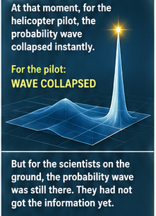
However, for the scientists on the ground, this collapse had not yet occurred. They had not received the image or positional data. In their model, the horse still existed as a distributed probability field across multiple regions of the forest. Only when the helicopter transmitted the photographic evidence and location data did their internal model update. At that exact moment, their probability distribution also collapsed into a single outcome.

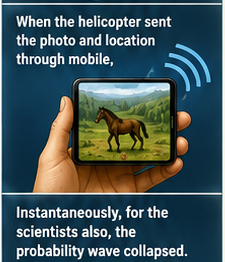
What is important is not the horse itself, but the structure of observation. The collapse appears instantaneous, almost infinitely fast, as if information has jumped across space without delay. But nothing physical is traveling faster than light. What changes is not matter or energy, but the state of knowledge—the internal probability representation held by each observer.

This leads to a deeper question: is this behavior unique to forests, animals, and human observation—or is it a more general feature of reality itself?

Because in quantum physics, an electron in a hydrogen atom is not described as a point moving along a fixed path.

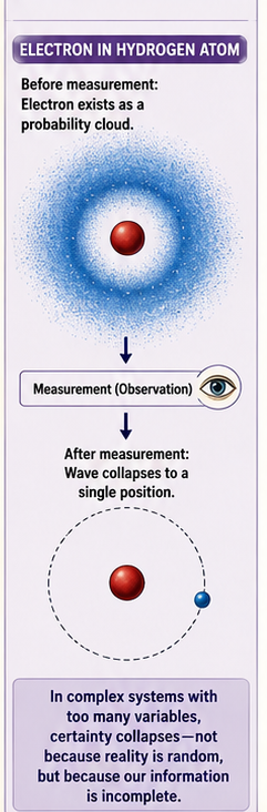
It is described as a probability cloud—a distributed wave of possible positions. Until measurement occurs, the electron does not have a single defined location in classical terms. It exists as a spatial probability distribution, much like the horse in the forest exists as a distributed probability wave in the scientists’ model.

The moment we measure the electron, the probability cloud appears to collapse into a single position. But just like in the forest, this collapse is not a physical object traveling across space—it is the transition from uncertainty to certainty within an observation frame. Different observers, with different access to information, effectively carry different versions of the same probability field until measurement or communication synchronizes them.

In this way, the forest becomes a large-scale visible analogy of something that also happens at the microscopic level. The horse represents a macroscopic system with hidden motion; the forest represents incomplete observation; the helicopter represents measurement; and the collapse represents information becoming complete within an observer’s frame.

The key idea of this entire system is this: probability is not just a measure of randomness, but a description of incomplete access to reality. And what we call “wave collapse” is not necessarily a physical destruction of possibilities, but a sudden alignment of information that turns a distributed probability field into a single experienced reality.

3] Insufficient Equations and the Birth of Probability

To understand why probability appears in science, we can begin with a simple contrast between fully determined and underdetermined systems.
First, consider the equation x+1=3x + 1 = 3x+1=3. Here, there is one unknown variable and one independent equation. The system is fully constrained, and it leads to a single definite solution: x=2x = 2x=2. There is no ambiguity, no alternative outcomes, and no need for probability. The system is complete, and the result is deterministic.
Now consider a different case: x + y=8x + y = 8x+y=8, where both x and y are positive integers. Here, there is only one equation but two unknown variables. This creates an underdetermined system, meaning there is not enough information to uniquely fix a single solution. Instead, multiple valid combinations exist.
We can list them clearly:

Each pair satisfies the same constraint x+y=8x + y = 8x+y=8, yet each represents a different valid state of the system. From a purely mathematical standpoint, none of these solutions is “wrong.” But from the perspective of an observer trying to predict a single outcome, there is no unique answer. The system allows a set of possibilities rather than a single result.
This is where probability naturally enters. When a system has more unknowns than independent constraints, we are forced to move from certainty to a distribution over possible solutions. Instead of one answer, we describe a space of answers. Probability becomes the language that represents this space when we do not have enough information to isolate a single point within it.

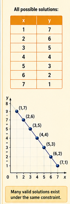
This idea connects directly to physical observation. In the forest analogy, the horse’s exact position cannot be solved from limited observations alone. Like the equation x+y=8x + y = 8x+y=8, there are many possible valid states consistent with the known constraints. The scientists therefore represent the horse not as a single point, but as a probability distribution across all possible locations.
In this way, probability is not necessarily a sign of randomness in the system itself, but a reflection of insufficient constraints in our description of it. When equations are complete, reality appears fixed. When equations are incomplete, reality appears distributed.
Thus, probability emerges as a bridge between limited information and full determinism—a structured way of representing all possible solutions when a single solution cannot yet be determined.

4] Too Many Variables and the Limits of Prediction (Weather System Analogy)

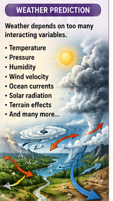
In simple systems, outcomes can be determined exactly because the number of known variables is sufficient to describe the system completely. However, in most real-world systems, the situation is fundamentally different. There are not just one or two variables, but an extremely large number of interacting variables, many of which are either partially known or completely unknown. In such cases, even though the system may still be deterministic in principle, prediction becomes practically impossible without switching to probability.
Weather prediction is one of the clearest examples of this situation. The weather of a region is not governed by a single factor, but by a massive interaction of temperature, pressure, humidity, wind velocity, ocean currents, solar radiation, terrain effects, and countless micro-scale atmospheric disturbances. Each of these variables changes continuously over time and interacts with others in nonlinear ways. Even a very small change in one parameter can amplify into large-scale differences in future conditions, a behavior commonly associated with complex dynamic systems.
Because of this extreme sensitivity and high dimensionality, it becomes impossible to write a complete set of equations that fully captures every influencing factor with perfect accuracy. Instead of a closed and solvable system, we are left with an open system containing too many variables and not enough precise constraints. This is exactly the same structural situation seen in the earlier examples, but at a much larger and more realistic scale.
As a result, weather prediction does not produce a single definite future state. Instead, it produces a probability distribution of possible future states. For example, instead of saying “it will definitely rain,” we say “there is a 70% chance of rain,” or “temperature will likely fall within a range.” These probabilities are not signs of randomness in nature alone, but reflections of incomplete knowledge of the full variable space governing the system.
In this sense, weather behaves like an expanded version of the equation x+y=8x + y = 8x+y=8, but with thousands or even millions of hidden variables instead of two. Since it is impossible to fully constrain the system, we replace exact prediction with statistical modeling. Probability becomes the only practical language capable of representing such high-dimensional uncertainty.
This leads to the deeper conclusion of Part 3: probability emerges not only from hidden variables or missing equations, but also from the overwhelming complexity of real systems. When the number of interacting variables becomes too large to fully measure or solve, certainty collapses—not because reality becomes random, but because our description of reality must shift from exact values to distributions of possibilities.
Thus, whether it is a horse moving through a forest, a simple equation with missing constraints, or the entire atmosphere shaping weather patterns, the underlying principle remains the same: probability is the mathematical response to insufficiently constrained systems in a world of overwhelming variables.

5] Another example of hidden variable – Mystery of feather in a room

Imagine a tiny feather floating in a room.

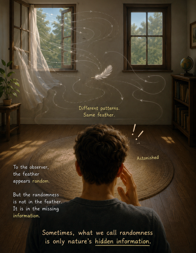
With two windows open, it follows one pattern. With one window open, it follows another.
To an observer who cannot feel the air currents, the feather appears random.
Probability maps can be created predicting where it may move next.
But the apparent randomness is not coming from the feather itself. It comes from missing information about the air flow.
This raises an interesting question:
When physicists describe an electron using probabilities, are those probabilities a complete description of reality, or could there be deeper information that remains hidden from observation?
Modern quantum mechanics generally treats the probability distribution as fundamental. However, the possibility of deeper underlying variables has fascinated scientists and philosophers since the early days of quantum theory.

Are probability waves describing reality itself, or are they describing our knowledge of reality?

beyond probability – Part-4 will be on still more interesting topics with examples.